Case Study Overview
Objective
Develop a production strategy for a small Brazilian fruit pulp company entering the European market. Use linear programming to determine the optimal production of soursop and cashew juice, balancing processing constraints, costs, and profitability. Apply different mathematical methods to validate the best solution and assess the impact of demand limitations.
Challenge
Optimizing production output while balancing processing constraints, cost efficiency, and profitability. Key challenges include managing limited processing capacity across two units, accounting for varying batch times per product, and maximizing profit margins (€7.50 for soursop vs. €4.50 for cashew). Additional complexities involve validating solutions using graphical, simplex, and Solver methods while assessing potential demand limitations.
Context
Brazil has great potential for expanding fruit cultivation, with the advantage of its geographical, climatic dimensions, and both domestic and international commercialization. The export of frozen fruit pulp from Brazil is still a little-explored market, with Brazilian exports mostly depending on requests from foreign importers. In this context, the Brazilian Export and Investment Promotion Agency (APEX-Brasil), in partnership with IBRAF, launched the "Brazilian Fruit" program in 1998, aiming at institutional and sales promotion to help companies meet the international market by directly connecting exporters with buyers.
Source: SANTOS, S. R. O.; KONDA, S. T. Export of fruit pulps: how a small company can participate in international trade. Revista Eletrônica Anima Terra, Mogi das Cruzes-SP, n. 3, p.1-11, 2016.
Case Study: Brasilidades
Brasilidades is a small fruit juice pulp industry that decided to invest in the European market. To this end, it decided to invest in producing soursop and cashew juice pulps, and as the production engineer of the company, you will be involved in the decision-making process regarding this new investment. You have found that in the production of these two new juices, there will be a need for two processing units: UPA and UPB. It was further noted that for producing ten liters of soursop juice, the process requires 8 minutes in UPA and 6 minutes in UPB to comply with export regulations. For producing ten liters of cashew juice, 4 minutes in UPA and 2 minutes in UPB are necessary, also to comply with export regulations. Brasilidades has a maximum processing availability of 480 for UPA and 200 for UPB per work shift. For the production of ten liters of the new juices, the total costs are €50 for soursop juice and €40 for cashew juice. On the other hand, the revenue from selling ten liters of the new juices is €57.50 for soursop juice and €44.50 for cashew juice.
Challenges to solve
a. Write the linear programming problem in its canonical form, considering the objective of achieving the highest profit margin from the production of soursop and cashew juices. Present all reasoning.
Initially organise the provided information before writing the equations:
Decision variables:
\( x_g = \text{quantity of 10L batches of Graviola juice} \)
\( x_c = \text{quantity of 10L batches of Cashew juice} \)
Profit margin per batch:
For 10L of Graviola juice = €57,50 - €50,00 = €7,50
For 10L of Cashew juice = €44,50 - €40,00 = €4,50
Constraints:
UPA availability = 480 min
UPB availability = 200 min
Production time for 10L Graviola juice: UPA = 8 min + UPB = 6 min
Production time for 10L Cashew juice: UPA = 4 min + UPB = 2 min
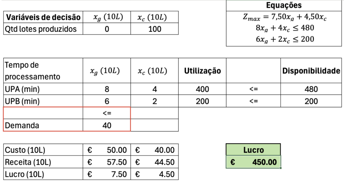
Objective function:
\[ \text{Maximise } (Z) = 7,50x_g + 4,50x_c \]
Subject to:
\[ 8x_g + 4x_c \leq 480 \]
\[ 6x_g + 2x_c \leq 200 \]
\[ x_g \geq 0 \text{ and } x_c \geq 0 \]
b. Use the graphical method and determine the optimal quantities of soursop and cashew juices to be produced per work shift. Present all calculations performed.
To solve using the graphical method, one must insert the constraints to identify the feasible region and use objective function level lines to find the optimal point.
1. Analyse constraints to determine feasible region
Regarding UPA:
\[ 8x_g + 4x_c \leq 480 \]
When \( x_g = 0 \):
\[ 8 \times 0 + 4x_c \leq 480 \]
\[ 4x_c \leq 480 \]
\[ x_c \leq 120 \]
Possible to produce 120 batches of 10L Cashew juice when not producing Graviola juice
When \( x_c = 0 \):
\[ 8x_g \leq 480 \]
\[ x_g \leq 60 \]
Possible to produce 60 batches of 10L Graviola juice when not producing Cashew juice
Regarding UPB:
\[ 6x_g + 2x_c \leq 200 \]
When \( x_g = 0 \):
\[ 2x_c \leq 200 \]
\[ x_c \leq 100 \]
Possible to produce 100 batches of 10L Cashew juice when not producing Graviola juice
When \( x_c = 0 \):
\[ 6x_g \leq 200 \]
\[ x_g \leq 33,333 \]
Possible to produce 33,333 batches of 10L Graviola juice when not producing Cashew juice
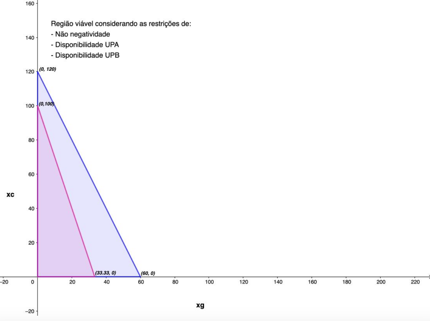
The pink region in the graph represents the feasible region with extreme points:
- \( (0, 0) \)
- \( (33,33, 0) \)
- \( (0, 100) \)
Substituting these points in the objective function:
\[ Z = 7,50x_g + 4,50x_c \]
Point (0, 0):
\[ Z = 7,50 \times 0 + 4,50 \times 0 = 0 \]
Point (33,33, 0):
\[ Z = 7,50 \times 33,33 + 4,50 \times 0 = 250 \]
Point (0, 100):
\[ Z = 7,50 \times 0 + 4,50 \times 100 = 450 \]
The highest value for the objective function was at point \( (0, 100) \), identifying it as the optimal solution. This indicates that producing 100 batches of 10L Cashew juice and no Graviola juice batches will yield €450,00 profit per work shift.
c. Use the simplex method to determine the optimal quantities of soursop and cashew juices to be produced per work shift. Present all calculations and interpret the last tableau.
- Insert slack variables in constraints:
\( 8x_g + 4x_c + x_{F1} = 480 \)
\( 6x_g + 2x_c + x_{F2} = 200 \) - Transform objective function:
\( Z = 7.50x_g + 4.50x_c \)
\( Z - 7.50x_g - 4.50x_c = 0 \) - Solution equations:
\( Z - 7.50x_g - 4.50x_c = 0 \)
\( 8x_g + 4x_c + x_{F1} = 480 \)
\( 6x_g + 2x_c + x_{F2} = 200 \) - Construct simplex tableau:
Z xg xc xF1 xF2 b F.O 1 -7.5 -4.5 0 0 0 1st R. 0 8 4 1 0 480 2nd R. 0 6 2 0 1 200 - Initial basic solution:
Assuming 0 for decision variables:
\( 8x_g + 4x_c + x_{F1} = 480 \)
\( x_{F1} = 480 - 8(0) - 4(0) \)
\( x_{F1} = 480 \)
\( 6x_g + 2x_c + x_{F2} = 200 \)
\( x_{F2} = 200 - 6(0) - 2(0) \)
\( x_{F2} = 200 \)
\( Z - 7.50(0) - 4.50(0) = 0 \)
\( Z = 0 \)
Non-basic variables: \( x_g = 0 \), \( x_c = 0 \)
Basic variables: \( x_{F1} = 480 \), \( x_{F2} = 200 \) - Determine entering/leaving variables:
\( 480/8 = 60 \) (1st row, xF1)Z xg xc xF1 xF2 b F.O 1 -7.5 -4.5 0 0 0 1st R. 0 8 4 1 0 480 2nd R. 0 6 2 0 1 200
\( 200/6 = 100/3 \) (2nd row, xF2)Z xg xc xF1 xF2 b F.O 1 -7.5 -4.5 0 0 0 1st R. 0 8 4 1 0 480 2nd R. 0 6 2 0 1 200 - Determine new basic solution:
Z xg xc xF1 xF2 b Pivot row 0 6 2 0 1 200 Row ÷6 0 1 0.333 0 0.1667 33.333 Z xg xc xF1 xF2 b New pivot 0 1 0.333 0 0.1667 33.333 ×7.5 0 7.5 2.5 0 1.25 250 Original F.O 1 -7.5 -4.5 0 0 0 New F.O 1 0 -2 0 1.25 250
Final tableau:Z xg xc xF1 xF2 b New pivot 0 1 0.333 0 0.1667 33.333 ×(-8) 0 -8 -2.666 0 -1.333 -266.666 1st R. 0 8 4 1 0 480 New 1st R. 0 0 1.333 1 -1.333 213.333
Non-basic: \( x_c = 0 \), \( x_{F2} = 0 \)Z xg xc xF1 xF2 b F.O 1 0 -2 0 1.25 250 1st R. 0 0 1.333 1 -1.333 213.333 2nd R. 0 1 0.333 0 0.1667 33.333
Basic: \( x_g = 33.333 \), \( x_{F1} = 213.333 \)
\( Z = 250 \) - Test new solution:
Z xg xc xF1 xF2 b New 1st row 1 0 -2 0 5/4 250 New 2nd row 0 0 4/3 1 -4/3 640/3 New 3rd row 0 1 1/3 0 1/6 100/3 Z xg xc xF1 xF2 b Pivot row 0 1 1/3 0 1/6 100/3 ×1/3 0 3 1 0 1/2 100 Z xg xc xF1 xF2 b New pivot 0 3 1 0 1/2 100 ×2 0 6 2 0 1 200 Z xg xc xF1 xF2 b Original 1st row 1 0 -2 0 5/4 250 New 1st row 1 6 0 0 9/4 450
Final optimal tableau:Z xg xc xF1 xF2 b New pivot 0 3 1 0 1/2 100 ×(-4/3) 0 -4 -4/3 0 -2/3 -400/3 2nd row 0 0 4/3 1 -4/3 640/3 New 2nd row 0 -1 0 1 -2 80
Non-basic variables: \( x_g = 0 \), \( x_{F2} = 0 \)Z xg xc xF1 xF2 b New 1st row 1 6 0 0 9/4 450 New 2nd row 0 -1 0 1 -2 80 New 3rd row 0 3 1 0 1/2 100
Basic variables: \( x_c = 100 \), \( x_{F1} = 80 \)
\( Z = 450 \)No negative coefficients in first row indicate optimal solution. Maximum profit of €450.00 achieved by producing 100 batches of cashew juice (xc) with 80 minutes remaining UPA availability per shift.
d. Use Excel's Solver and determine the optimal quantities of soursop and cashew juices to be produced per work shift. Present a "print" of the spreadsheet used.

According to Solver: Maximum profit of €450.00 requires 100 batches of cashew juice and 0 batches of graviola juice. Remaining 80 minutes UPA availability per shift.
e. What is the highest contribution margin, in euros, obtained from the production of the two new juices in one work shift? Present your reasoning and calculations.
f. Now suppose that the demand for soursop juice is limited to 400 liters per shift. Does adding this new constraint change the solution obtained in items (b) and (e)? If yes, present the new solution with calculations. If no, justify your answer with calculations.
Key Results
Optimal Production Plan
- 100 batches of cashew juice (10L each)
- 0 batches of soursop juice
- Remaining capacity: 80 UPA minutes
Financial Outcomes
- Maximum profit: €450/shift
- Equivalent to R$2,720.33 (€1 = R$6.04)
- 44.4% higher than alternative configurations