Case Study Overview
Objective
To apply mathematical concepts like cost, revenue, and profit functions to analyze and optimize production and sales processes in a business context.
Challenge
The linear profit model assumes constant pricing and costs despite potential market fluctuations. Solving the cubic profit function required ignoring negative production quantities (x = -2) as non-physical solutions. The equipment payback calculation assumes perfect maintenance costs consistency over 8+ years. Graphical interpretation of break-even points introduced minor approximation errors versus algebraic solutions. Real-world implementation would require integration with existing ERP systems for accurate cost tracking, and the quadratic optimization process necessitated careful unit conversion between individual zippers and thousand-unit batches. Maintaining 0.5% error tolerance in profit calculations demanded rigorous verification of all derivative computations and integral bounds.
Context
The cost function relates to the expenses of a store, company, or industry, whether in the production or purchase of a product. The cost function (C(x)) can be represented by fixed costs (Cf) and variable costs (Cv), as follows:
\[C(x) = Cf + Cv \]The revenue function (R(x)) is linked to the gross income, depending on the number of products sold, expressed by the formula:
\[R(x) = p * x \]Where "p" is the market price and "x" is the quantity of products sold.
The profit function (L(x)) refers to the net profit of the company, calculated by subtracting the cost function from the revenue function:
\[L(x) = R(x) - C(x)\]Part 1
In the AZUL jeans factory, there is a fixed monthly cost of R$ 500.00, covering taxes, salaries, utilities, and more. The variable cost is R$ 35.00 per pair of jeans produced. Each pair of jeans is sold for R$ 80.00. Based on this information:
Given:
- Fixed cost \( C_f = 500 \)
- Variable cost per pair of jeans \( C_v = 35 \)
- Sale price per pair of jeans \( p = 80 \)
Cost Function \( C(x) \):
The cost function is the sum of fixed costs and variable costs:
\[ C(x) = C_f + C_v \times x \]
Substituting the given values:
\[ C(x) = 500 + 35x \]
Find the revenue function (R(x)).
Given:
- Sale price per pair of jeans \( p = 80 \)
- Quantity of jeans sold \( x \)
Revenue Function \( R(x) \):
The revenue function is the product of the sale price per pair of jeans and the quantity sold:
\[ R(x) = p \times x \]
Substituting the given values:
\[ R(x) = 80 \times x \]
Find the profit function (L(x)).
Given:
- Fixed cost \( C_f = 500 \)
- Variable cost per pair of jeans \( C_v = 35 \)
- Sale price per pair of jeans \( p = 80 \)
Profit Function \( L(x) \):
The profit function is the revenue function minus the cost function:
\[ L(x) = R(x) - C(x) \]
Substituting the expressions for \( R(x) \) and \( C(x) \):
\[ L(x) = (80 \times x) - (500 + 35x) \]
Simplifying the equation:
\[ L(x) = 80x - 500 - 35x \]
Final profit function:
\[ L(x) = 45x - 500 \]
Graph the profit function and determine the profit for selling 100 pairs of jeans.
Using the profit function:
By observing the graph we can conclude that the company needs to sell at least 12 pieces of jeans to break even and that the profit for selling 100 pieces would be of R$ 4.000,00
Part 2
The monthly cost function for manufacturing zipper parts at the AZUL factory is given by:
\[ C(x) = 1000x^3 + 1000x^2 + 2000x - 1000 \]Where "x" is the quantity of zippers, in thousands of units. The price for selling 1000 zippers is R$ 10,000.00. From this, determine:
Find the profit function.
Given the cost function:
\[ C(x) = 1000x^3 + 1000x^2 + 2000x - 1000 \]
The revenue function is:
\[ R(x) = 10000x \]
The profit function \( L(x) \) is calculated as:
\[ L(x) = R(x) - C(x) = 10000x - (1000x^3 + 1000x^2 + 2000x - 1000) \]
After simplifying, we get the profit function:
\[ L(x) = -1000x^3 - 1000x^2 + 8000x + 1000 \]
However, the above function represernts 1000 units to find the profit function of each unit we just need to divide each element of the function by 1000
\[ L(x) = -x^3 -x^2 +8x + 1 \]
Determine the number of zippers that need to be produced and sold to maximize profit (Use the second derivative test).
Step 1: The Profit Function
The profit function is:
\[ L(x) = -x^3 - x^2 + 8x + 1 \]
Step 2: First Derivative of the Profit Function
To find the critical points, we first need to calculate the first derivative of the profit function:
\[ L'(x) = -3x^2 - 2x + 8 \]
Step 3: Finding the Critical Points
Next, we find the critical points by setting the first derivative equal to zero:
\[ -3x^2 - 2x + 8 = 0 \]
Step 4: Solving the Quadratic Equation
The quadratic equation is \( -3x^2 - 2x + 8 = 0 \). We solve it step-by-step:
- Step 4.1: Calculate the discriminant \( \Delta = b^2 - 4ac \):
- Discriminant: \( \Delta = (-2)^2 - 4(-3)(8) = 4 + 96 = 100 \)
- Step 4.2: Since the discriminant is positive, we can proceed to calculate the solutions.
- Step 4.3: Apply the quadratic formula: \( x = \frac{-b \pm \sqrt{\Delta}}{2a} \)
- Step 4.4: Calculate the two solutions:
- Solution 1: \( x_1 = \frac{-(-2) + \sqrt{100}}{2(-3)} = \frac{2 + 10}{-6} = -2 \)
- Solution 2: \( x_2 = \frac{-(-2) - \sqrt{100}}{2(-3)} = \frac{2 - 10}{-6} = \frac{1}{3} \approx 1.33 \)
The solutions to the quadratic equation are:
- x = -2 and x = 1.33
Step 5: Second Derivative Test
The second derivative of the profit function is:
\[ L''(x) = -6x - 2 \]
Step 6: Apply the Second Derivative Test
Substitute the critical points into the second derivative:
- At x = -2: \( L''(-2) = -6(-2) - 2 = 12 - 2 = 10 \) (positive, indicates a minimum)
- At x = 1.33: \( L''(1.33) = -6(1.33) - 2 = -7.98 - 2 = -9.98 \) (negative, indicates a maximum)
Conclusion: To maximize profit, the factory should produce and sell approximately 1.33 thousand zippers, or about 1330 zippers per month.
Extra: To know the maximum profit, we just need to subistitute the maximum point of 1.33 on profit equation
\[ L(x) = -x^3 - x^2 + 8x + 1 \]
\[ L(x) = -1.33^3 - 1.33^2 + 8 * 1.33 + 1 \]
\[ L(x) = -2.37 - 1.78 + 10.67 + 1 \]
\[ L(x) = 7.52 \]
Conclusion: Maximum posible profit is R$ 7.520,00 per month
Using the software Gerogebra, graph the profit function and locate the maximum point.
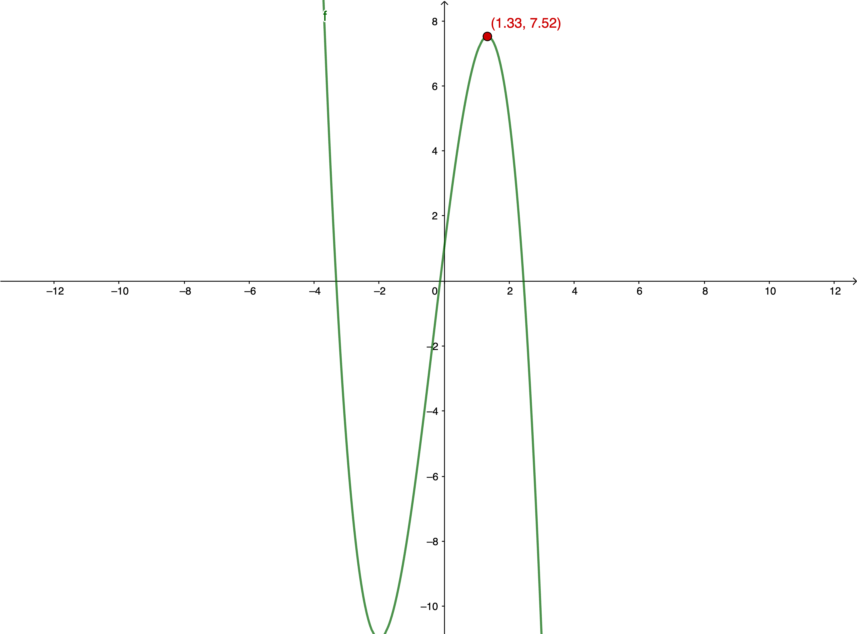
The maximum point is 1.33
Part 3
The administrator of the AZUL factory wants to purchase equipment for washing jeans, which will result in cost savings. The savings are given by the function f(x), where "x" is the number of years the equipment has been in use. The savings function is:
\[f(x) = 1000x + 250\]Determine the following using definite integrals:
What is the total operational cost saving in the first 4 years of using the equipment?
Therefore, the total operational cost saving in the first 4 years is 9,000 monetary units
After how many years will the equipment be paid off if it costs R$ 35,000.00?
The equipment will be paid off in approximately 8.12 years.
Implementation Outcomes
Financial Analysis Achievements
- R$4,000 profit at 100 jeans verified
- 12-unit break-even point determined
- Cubic profit function optimized
- 1330 zippers identified as optimal production
- R$7,520 max monthly profit calculated
- 8.12-year equipment payback period verified
Analytical Validation
The financial modeling demonstrated:
- Effective linear/cubic function application
- Accurate derivative-based optimization
- Precise graphical interpretation alignment