Optimizing Warehouse Logistics: A Mathematical Approach

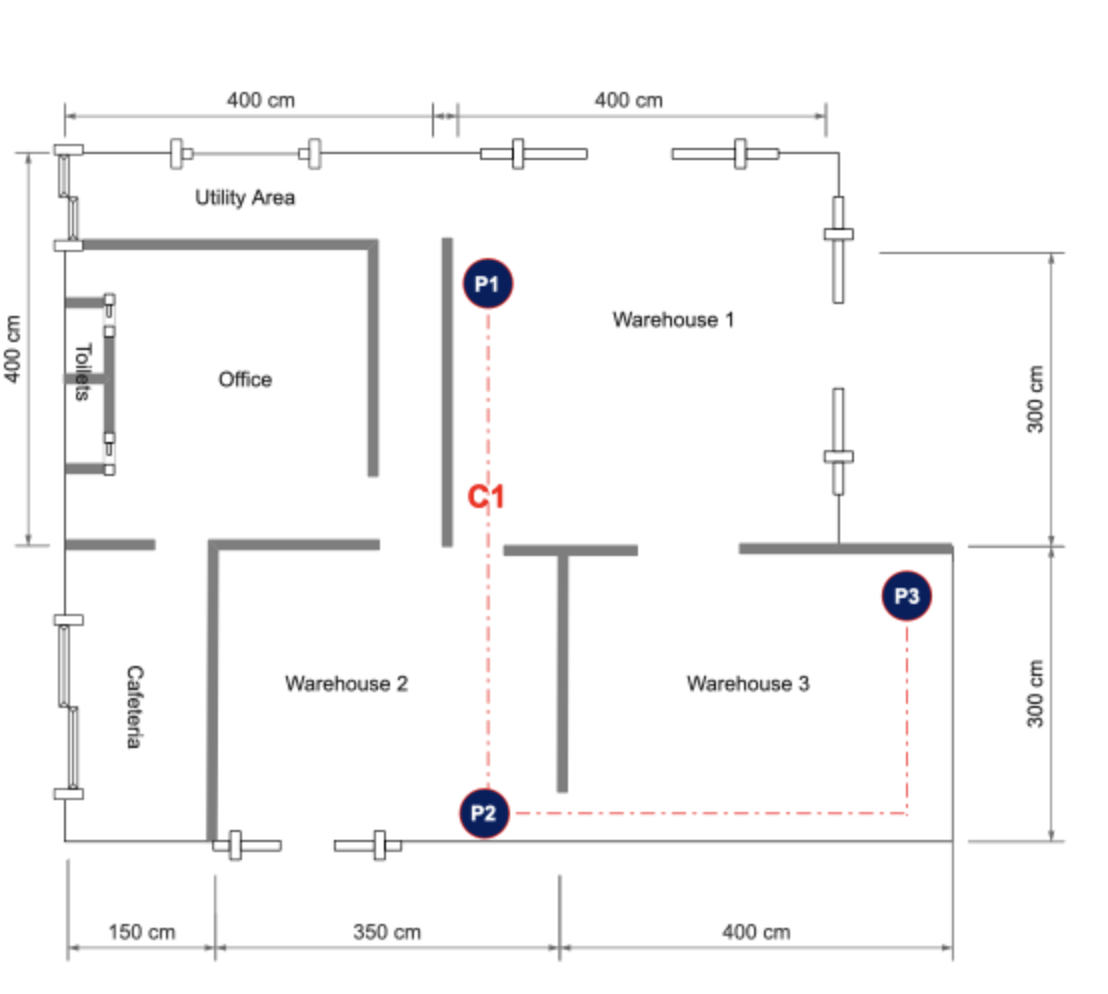
Imagine you are a trainee at a company that distributes mechanical parts, Distributor X. In one of the routine meetings, management presented a new project, which involves the installation of new conveyor belts in one of its warehouses. One belt would connect warehouse 1 to warehouse 2 and the second would connect warehouse 2 to warehouse 3, making the necessary structural changes.

The warehouse is presented as follows:

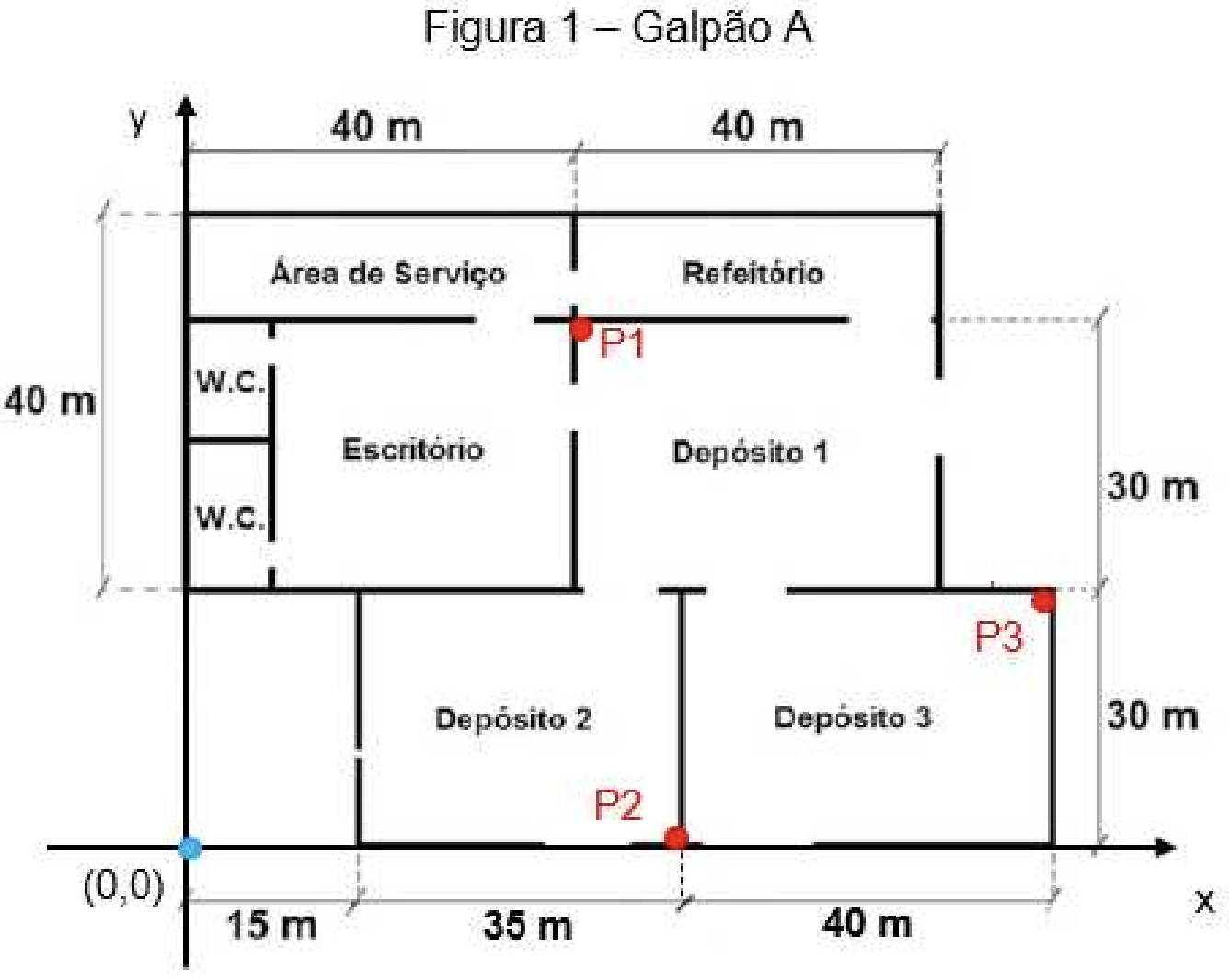
You were involved in the project to assist in the initial estimates. Considering that the belts have no elevation, that Belt I starts at position P1 and ends at P2, and that Belt II starts at P2 and ends at P3:

1. What is the length of Belt I?

Given:

• P1 (40, 60)
• P2 (50, 0)

\[d_{AB} = \sqrt{(x_1 - x_2)^2 + (y_1 - y_2)^2}\] \[d_{P1 P2} = \sqrt{(40 - 50)^2 + (60 - 0)^2}\] \[d_{P1 P2} = \sqrt{(-10)^2 + (60)^2}\] \[d_{P1 P2} = \sqrt{100 + 3600}\] \[d_{P1 P2} = \sqrt{3700}\] \[d_{P1 P2} = 60.82\]

The length of the belt I is 60.82 m.

2. What is the length of Belt II?

Given:

• P2 (50, 0)
• P3 (90, 30)

\[d_{AB} = \sqrt{(x_1 - x_2)^2 + (y_1 - y_2)^2}\] \[d_{P2 P3} = \sqrt{(50 - 90)^2 + (0 - 30)^2}\] \[d_{P2 P3} = \sqrt{(-40)^2 + (-30)^2}\] \[d_{P2 P3} = \sqrt{1600 + 900}\] \[d_{P2 P3} = \sqrt{2500}\] \[d_{P2 P3} = 50\]

The length of the belt II is 50 m.

3. If a third belt "Belt III" were needed, connecting P1 to P3, what size would it be?

Given:

• P1 (40, 60)
• P3 (90, 30)

\[d_{AB} = \sqrt{(x_1 - x_2)^2 + (y_1 - y_2)^2}\] \[d_{P1 P3} = \sqrt{(40 - 90)^2 + (60 - 30)^2}\] \[d_{P1 P3} = \sqrt{(-50)^2 + (-30)^2}\] \[d_{P1 P3} = \sqrt{2500 + 900}\] \[d_{P1 P3} = \sqrt{3400}\] \[d_{P1 P3} = 58.3\]

If there was a third belt connecting P1 to P3 its length would be 58.3 m.

The idea of installing these new belts motivated new actions, including the interconnection of the various warehouses of the company, with the aim of optimising the transport time of items from one to another.

The following are the warehouses and the possible flows of transport of mechanical parts.

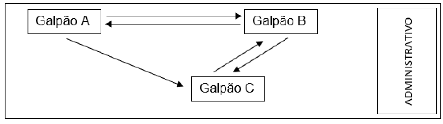
In situations like this, we can use a matrix to simulate the inter-relationship between the warehouses. Your supervisor would like you to analyse the flows between the warehouses using matrices and, as an example, he presented the following situation:

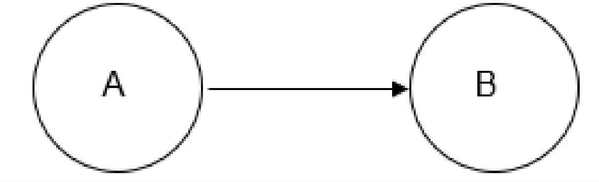
This situation can be represented as a matrix, where, in the first row, the connections between A and other points are presented and in the second row, the connections between B and other points are presented. If there is a flow, the element in the matrix will be 1, if there is no flow, the element will be zero. Thus, as there are two positions, a 2x2 matrix must be considered:

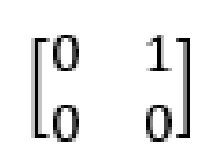
It can be seen that A does not connect with itself, therefore the element of the first row/first column will be zero, but it will be 1 in the second row, as there is a flow from A to B. Position B has no flow leading to any position.

1. Present matrix A, which represents the flows of parts between the warehouses.

Considering that we have 3 warehouses and three possible flows of parts, we will have a square matrix of order 3. Where the first row represents warehouse A, the second row represents warehouse B, and the third row represents warehouse C. And the first column represents the flow of parts to warehouse A, the second column represents the flow of parts to warehouse B, and the third column represents the flow of parts to warehouse C, we have the following matrix:

\[A_{(3X3)} = \begin{bmatrix} 0 & 1 & 1 \\ 1 & 0 & 1 \\ 0 & 1 & 0 \end{bmatrix}\]
2. Present matrix D, which represents the total quantities of demands, in millions of units, defined by matrix A multiplied by matrix M.

\[A * M = D\]

\[\begin{bmatrix} 0 & 1 & 1 \\ 1 & 0 & 1 \\ 0 & 1 & 0 \end{bmatrix} \begin{bmatrix} 0 & 1 & 2 \\ 1 & 0 & 2 \\ 1 & 2 & 0 \end{bmatrix} = \begin{bmatrix} 2 & 2 & 2 \\ 1 & 3 & 2 \\ 1 & 0 & 2 \end{bmatrix}\]

\[d_{11} = 0 * 0 + 1 * 1 + 1 * 1 = 2\] \[d_{12} = 0 * 1 + 1 * 0 + 1 * 2 = 2\] \[d_{13} = 0 * 2 + 1 * 2 + 1 * 0 = 2\] \[d_{21} = 1 * 0 + 0 * 1 + 1 * 1 = 1\] \[d_{22} = 1 * 1 + 0 * 0 + 1 * 2 = 3\] \[d_{23} = 1 * 2 + 0 * 2 + 1 * 0 = 2\] \[d_{31} = 0 * 0 + 1 * 1 + 0 * 1 = 1\] \[d_{32} = 0 * 1 + 1 * 0 + 0 * 2 = 0\] \[d_{33} = 0 * 2 + 1 * 2 + 0 * 0 = 2\]


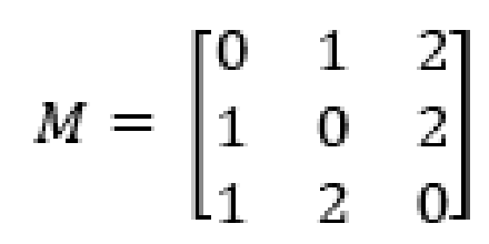
The D matrix representing the quantities of demand in millions of units is:

\[D = \begin{bmatrix} 2 & 2 & 2 \\ 1 & 3 & 2 \\ 1 & 0 & 2 \end{bmatrix}\]

There is a way to calculate the occupancy of each warehouse, using the D demand matrix, which corresponds to the answer to question 2 of Part 2.

To do this, it is first necessary to calculate the eigenvalues of matrix D. Then choose the eigenvector that corresponds to the highest eigenvalue among the calculated eigenvalues. Divide each coordinate of the eigenvector by the sum of its coordinates. The values found will correspond to the occupancy of the warehouses, respectively, of Warehouse A, Warehouse B and Warehouse C.

1. Calculate the eigenvalues of matrix D.
\[D = \begin{bmatrix} 2 & 2 & 2 \\ 1 & 3 & 2 \\ 1 & 0 & 2 \end{bmatrix}\]

\[P_{(\lambda)}= det{(D - \lambda I)}= \begin{bmatrix} 2 - \lambda & 2 & 2 & 2 - \lambda & 2\\ 1 & 3 - \lambda & 2 & 1 & 3- \lambda\\ 1 & 0 & 2 - \lambda & 1 & 0 \end{bmatrix}=0\] \[det{(D - \lambda I)}= (2 -\lambda) * (3 -\lambda) * (2 -\lambda) + 4 + 0 -2(3 -\lambda) -0 -2(2 -\lambda) = 0\] \[det{(D - \lambda I)}= \lambda^2 -5\lambda +6(2 -\lambda) + 4 -6 +2\lambda -4 + 2\lambda = 0\] \[det{(D - \lambda I)}= -\lambda^3 +2\lambda^2 -10\lambda + 5\lambda^2 +12 - 6\lambda -2 + 4\lambda -4 = 0\] \[det{(D - \lambda I)}= -\lambda^3 +7\lambda^2 -12\lambda + 6 = 0\]


\[P{(\lambda)}=0 \Rightarrow -\lambda^3 +7\lambda^2 -12\lambda + 6 = 0\]


1, 2, 3 or 6 are the roots of this polynomial. Replacing the λ values:

\[-(1)^3+7*(1)^2-12*1+6=0\] \[-1+7-12+6=0\] \[-13+13 = 0\]

Therefore 1 is the root of the polynomial. Applying Briot-Ruffini's rule (Ruffini's synthetic division):




	-1	7	-12	6
1		-1	6	-6
	-1	6	-6	0
=	\[-\lambda^2\]	\[6\lambda\]	\[-6\]	\[0\]




Now that we have a second-degree polynomial, we just need to apply the quadratic equation.

\[\Delta = b^2-4ac\] \[\Delta = 6^2-4(-1)(-6)\] \[\Delta = 36-24\] \[\Delta = 12\]
\[x=\dfrac{-b \pm \sqrt\Delta}{2a}\] \[x=\dfrac{-6 \pm \sqrt12}{2(-1)}\] \[x=\dfrac{-6 \pm 2\sqrt3}{-2}\] \[x=-3 \pm \sqrt3\]


The eigenvalues are: 1, 3+√3, 3-√3 or, solving the squareroots: 1, 4.73, 1.27

2. Find the maximum eigenvalue.

The maximum eigenvalue is 4.73. It was calculated on the previous question.

3. Present the eigenvector of the eigenvalue calculated in (2).
\[D=\begin{bmatrix} 2 & 2 & 2 \\ 1 & 3 & 2 \\ 1 & 0 & 2 \end{bmatrix} -\begin{bmatrix} 4.7 & 0 & 0 \\ 0 & 4.7 & 0 \\ 0 & 0 & 4.7 \end{bmatrix} = \begin{bmatrix} -2.7 & 2 & 2 \\ 1 & -1.7 & 2 \\ 1 & 0 & -2.7 \end{bmatrix}\]

\[(A - \lambda I)=\begin{bmatrix} -2.7 & 2 & 2 \\ 1 & -1.7 & 2 \\ 1 & 0 & -2.7 \end{bmatrix} \begin{bmatrix} x \\ y \\ z \end{bmatrix} = 0\]




The matrix brings us to the system of linear equations below:

\begin{align*} -2.7x + 2y + 2z&= 0 \\ x - 1.7y +2z &= 0 \\ x - 2.7z &= 0 \end{align*}

Isolating one of the equations:

\[x - 2.7z =0\] \[x =2.7z\]

Substituting the new x in one of the equations:

\[-2.7x + 2y + 2z= 0\] \[-2.7(2.7z) + 2y + 2z= 0\] \[-7.4z + 2y + 2z= 0\] \[-5.4z + 2y = 0\] \[2y=5.4z\] \[y=\frac{5.4z}{2}\] \[y=2.7z\]


The eigenvector is: 2.7, 2.7, 1

4. Calculate the occupancies of each warehouse.

o determine the occupancy of each warehouse, we divide each component of the calculated eigenvector by the sum of all components. Each component corresponds to a specific warehouse.




eigenvector: (2.7, 2.7, 1)

sum of the coordinates: 2.7 + 2.7 + 1 = 6.5

\[A=\frac{2.7}{6.5} = 0.415 = 41.5\%\] \[B=\frac{2.7}{6.5} = 0.415 = 41.5\%\] \[C=\frac{1}{6.5} = 0.153 = 15.3\%\]


Occupancy of the warehouse A and B is of 41.5% and the C is of 15.3%

It is intended, to carry out all the intended adjustments, to buy materials A, B and C for the construction and modification of the structure. Knowing that the cost of A is R$50.00, the cost of B is R$70.00 and the cost of C is R$30.00, consider:

• The cost involved in the purchase of A and B must be R$17,000.00
• The cost involved in the purchase of B and C must be R$16,000.00
• The cost involved in the purchase of A and C must be R$19,000.00

1. What are the quantities of each material to be purchased?

Using the information provided, we can build the linear equations and matrices to solve the exercise

\begin{align*} 50a + 70b &= 17000 \\ 70b + 30c &= 16000 \\ 50a + 30c &= 19000 \end{align*}

\[\begin{aligned} \begin{bmatrix} 50 & 70 & 0 \\ 0 & 70 & 30 \\ 50 & 0 & 30 \end{bmatrix} \begin{bmatrix} a \\ b \\ c \end{bmatrix} &= \begin{bmatrix} 17000 \\ 16000 \\ 19000 \end{bmatrix} \end{aligned}\]

\[\begin{aligned} \begin{bmatrix} 50 & 70 & 0 & 50 & 70\\ 0 & 70 & 30 & 0 & 70\\ 50 & 0 & 30 & 50 & 0 \end{bmatrix} \end{aligned}\]

\[0-0-0+105000+105000+0 = 210000 \Rightarrow det_{C}=210000\]

\[\begin{aligned} \begin{bmatrix} 17000 & 70 & 0 & 17000 & 70\\ 16000 & 70 & 30 & 16000 & 70\\ 19000 & 0 & 30 & 19000 & 0 \end{bmatrix} \end{aligned}\]

\[0-0-33600000+35700000+39900000+0 = 42000000 \Rightarrow det_{Ca}=42000000\]

\[\begin{aligned} \begin{bmatrix} 50 & 17000 & 0 & 50 & 17000\\ 0 & 16000 & 30 & 0 & 16000\\ 50 & 19000 & 30 & 50 & 19000 \end{bmatrix} \end{aligned}\]

\[0-28500000+0+24000000+25500000+0 = 21000000 \Rightarrow det_{Cb}=21000000\]

\[\begin{aligned} \begin{bmatrix} 50 & 70 & 17000 & 50 & 70\\ 0 & 70 & 16000 & 0 & 70\\ 50 & 0 & 19000 & 50 & 0 \end{bmatrix} \end{aligned}\]

\[-59500000-0-0+66500000+56000000+0 = 63000000 \Rightarrow det_{Cc}=63000000\]


\[a=\frac{42000000}{210000} \Rightarrow 200\] \[b=\frac{21000000}{210000} \Rightarrow 100\] \[c=\frac{63000000}{210000} \Rightarrow 300\]

Quantities to be purchased:

• Product a: 200 units.
• Product b: 100 units.
• Product c: 300 units.

2. Considering the quantities found in (1), if the cost of the three materials were R$50.00, what would be the total cost?

Considering the same cost price for all three products, just need to multiply the cost price per quantity. I will call the price the constant k and each product as a, b, and c to formulate the problem mathematically:

\[Cost= k(a+b+c)\]

Substituting the numbers

\[Cost=50(200+100+300)\] \[Cost=50(600)\] \[Cost=30000\]

The cost would be of R$ 30000,00